Machine Learning with Python - Part 2

This tutorial assumes that you’ve thoroughly gone through the previous tutorial where we covered the basics of machine learning. You won't be able to follow the guidelines described here without going through the previous article Machine Learning with Python.

Expectations from this tutorial

In the last tutorial we learned about Machine Learning, its importance and influence on our everyday lives, and its potential future impacts. We also learned about installing and importing different libraries used for machine learning and data pre processing. We will use data to train the machine using different algorithms. Different models for machine learning will be used to train the machine and we will predict by querying our machine.

Importing the Training Data

It goes without saying that first we have to train our model (Machine Learning algorithm) and make sure of our baseline preparation to make it able to perform in the appropriate conditions.

The dataset we will be working with in this tutorial is one of the well-known datasets called Iris Flower Dataset from UC Irvine Machine learning repository link. UC Irvine repository contains thousands of the datasets freely available to train your machine and perform analysis. We will be using Iris Flower Dataset, a multivariate dataset that holds 150 observations (records). To know more about this visit Wikipedia.

First we include our required libraries

import pandas

from pandas.tools.plotting import scatter_matrix

import matplotlib.pyplot as plt

from sklearn import model_selection

from sklearn.metrics import classification_report

from sklearn.metrics import confusion_matrix

from sklearn.metrics import accuracy_score

from sklearn.linear_model import LogisticRegression

from sklearn.tree import DecisionTreeClassifier

from sklearn.neighbors import KNeighborsClassifier

from sklearn.discriminant_analysis import LinearDiscriminantAnalysis

from sklearn.naive_bayes import GaussianNB

from sklearn.svm import SVC

After successfully importing the desired libraries we now load the dataset.

Note: As this is the hello world set of machine learning, it is already included in machine learning repositories.

You need to make sure that when you execute the above code, you receive no errors. If some errors do pop up, go back and check what errors you’re facing? You can describe the error below in the comment section and I will be happy to assist.

To load our code in python use the following code:

url = "https://archive.ics.uci.edu/ml/machine-learning-databases/iris/iris.data"

names = ['sepal-length', 'sepal-width', 'petal-length', 'petal-width', 'class']

dataset = pandas.read_csv(url, names=names)

You can also include the dataset by grabbing it from here and saving it in your working directory. If you follow the latter method make sure to change the url to that local directory containing the dataset.

Now, let’s move forward to gain some information about the dataset.

We can have a quick look at how many observations (rows) and attributes (columns) our dataset consists of by using this simple command:

print(dataset.shape)

This command returns the result as

(150, 5)

which shows our dataset has 150 rows and 5 columns.

Afterwards, it’s good practice to have a quick glimpse at your data. We will do it with the help of the head command which returns the number of records passed to it in through parameters.

print(dataset.head(20))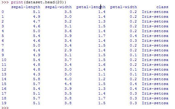

The head function returned the first 20 records of the data out of 150.

Next, we’ll inspect the statistical summary of our data which includes count, minimum, mean, maximum values as well as some percentiles. Sklearn library contains the describe function which performs and returns different statistics.

print(dataset.describe())

Build Model

Now that you’re familiar with the dataset, it’s time to train our machine and build a model which will predict and give results.

There are multiple algorithms available which can be used to train our machine. In this tutorial, we will use Logistic Regression (LR) and K-Nearest Neighbour (KNN) to train our machine. Later, we will make some predictions on the data and these results will be compared to find which model has the more accuracy using the above data. I chose LR and KNN randomly, you can use other models to build your models (Naive Bayes, KNN…) by using any dataset.

Before we start actually building our model though, we need to make some validation proof of these models we are going to build.

So, we are going to hold back some data from our dataset that will be unseen for the machine. Later, this data will be given to the model to predict the outcomes of the missing attributes.

# Split-out validation dataset

array = dataset.values

X = array[:,0:4]

Y = array[:,4]

validation_size = 0.20

seed = 7

X_train, X_validation, Y_train, Y_validation = model_selection.train_test_split(X, Y, test_size=validation_size, random_state=seed)



seed = 7

scoring = 'accuracy'

Now, let’s build our model using the mentioned modeling algorithms.

models = []

models.append(('LR', LogisticRegression()))

models.append(('KNN', KNeighborsClassifier()))

We called both of the models and saved them in an array of model. We will access both of the models using the foreach loop to train the machine using our dataset.

results = []

names = []

for name, model in models:

    kfold = model_selection.KFold(n_splits=10, random_state=seed)

    cv_results = model_selection.cross_val_score(model, X_train, Y_train, cv=kfold, scoring=scoring)

    results.append(cv_results)

    names.append(name)

    msg = "%s: %f (%f)" % (name, cv_results.mean(), cv_results.std())

    print(msg)

The code above will  train our machine based upon the two models we defined in the models array. It will show you the accuracy of both models as an input where you can compare them both and choose a single one for further processing.

Our output contains both of the model’s accuracy. We can see that KNN has the more accuracy compare to the LR model.

So, we will take KNN as our final mode and will make some predictions on it.

Make Predictions

As KNN happens to be the best algorithm for our model, we will know the accuracy of the model on our validation dataset which we separated from the dataset earlier.

knn = KNeighborsClassifier()

knn.fit(X_train, Y_train)

predictions = knn.predict(X_validation)

print(accuracy_score(Y_validation, predictions))

print(confusion_matrix(Y_validation, predictions))

print(classification_report(Y_validation, predictions))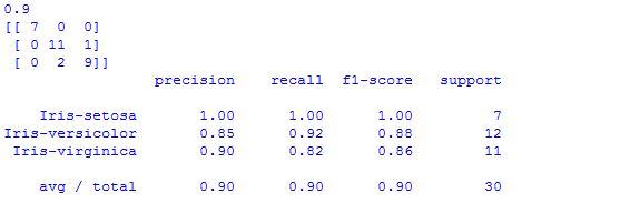

Conclusion

We can see that our designed model is 0.9 or 90% accurate. The confusion matrix shows the indication of the three errors made. At the end, the classification report contains the  precision, recall, f1-score and support shows the excellent result.

Hope you enjoyed. Feel free to leave questions in the comments.

Be sure to stop by DiscoverSDK for the best development tools.